📘
This article is also available in PDF format.

Introduction#

In this paper we explore how to improve the subpixel linearity of Intel RealSense Depth Camera D400 series. We will introduce a new “Advanced Depth Parameter” that we call the A-factor, that can be used to tune and improve the subpixel linearity by a factor of 3-5x, i.e. linearity of depth measurements between discrete disparities. To explain this, we digress briefly to the fundamentals underpinning the calculation of depth from stereo. Stereo depth cameras consist of two fixed cameras pointing in the same direction, but separated by a certain distance, called the baseline. The left and right images captured by these cameras are compared on a per-frame basis in order to determine which parts of simultaneously captured images match up. This is also known as solving the correspondence problem. Objects that are close will experience a larger shift, along the axis defined by the two imagers, than objects that are far away. This means that every pixel in the right image would need to be shifted by a different amount to match the proper left image pixel, depending on its distance away, or range. The local shifts are quantified as a number of pixels shifted and is known as the disparity. Finally, through triangulation it is possible to relate the disparity shift of every pixel to the range to every point in the image.

Depth is consequently derived from this equation:

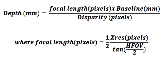
Where Xres is the horizontal resolution of the imager (for example 848 or 1280). HFOV is the horizontal field of view which is 90° for Model D435 and 65° for Model D415.

In order to determine the depth resolution or minimum step-size of the depth, one can differentiate with respect to the disparity, to get:

The key observation from this equation is that the depth resolution will be determined by the smallest step size of the Disparity, DisparityStep. We also call this the Subpixel. Normally one would assume that this is 1 pixel. However, stereo depth algorithms are often judged by the size of the “subpixel resolution” that they are able to achieve. A state-of-the-art algorithm such as that which is inside the D4 ASIC in the Intel RealSense D4xx Depth Cameras may, for example, have 1/32 pixel resolution. However, achieving this small subpixel involves a series of non-trivial image operations, and has been the subject of much research.

In this paper we characterize the subpixel linearity of existing Intel RealSense Depth Camera D415 and D435 models, and introduce a new “Advanced Depth Parameter”, called the A-factor, that can be adjusted to improve this linearity. This is an on-chip parameter so it has no effect on bandwidth or power consumption on the host, but it is volatile, so when the unit loses power it will revert to the current default A-factor value of 0. This subpixel linearity is not to be confused with calibration which can change the overall slope or off-set of depth measurements over larger distances.

Measurement and tuning of Subpixel Linearity#

Let us start by considering a controlled experiment of pointing a D435 at a textured flat wall, and then move the camera away from the wall while measuring the depth with the on-chip stereo algorithm (y-axis) as a function of known distance from the wall, aka the target range or ground truth (x-axis).

In this example we show the results for two different depth settings:

The “High Density” depth setting.
The “High Accuracy” preset.

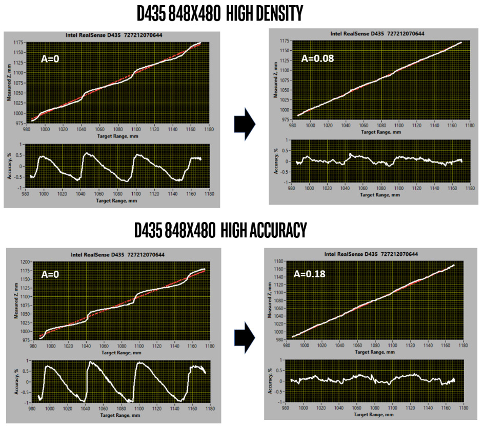
944 — Figure 1. Shows the subpixel depth linearity for “High Density” (top) and “High Accuracy” (bottom) depth presets, comparing D435 performance for the default A=0 (left) versus an optimized value for A (right). The accuracy curves plot the deviation from linearity, and show an oscillatory behavior between discrete disparities. In the measurements above, the distance range was chosen to cover about 3 disparities.

The first thing we notice is that for both depth settings the depth measurements are NOT linear and instead show clear oscillations of about +/-0.5% at the measured range (~1m) for the “High density” preset, and about twice that for the “High Accuracy”. However, we also see that with proper choice of the new A-factor in the advanced settings, it is possible to greatly improve the linearity, reducing the amplitude of deviation by 3-4x.

As noted, the optimum A-factor is different for different depth presets. We have investigated a set of different targets and determined that the optimal value is fairly independent of scene texture as well as whether it is active illumination (with projector on) or passive (with projector off). There is some minor dependence on resolution. We have created a table below of what we recommend as optimal values for each preset. The main observation is that with the exception of the “High accuracy” depth settings, a value of 0.08 across the board would greatly improve the depth linearity.

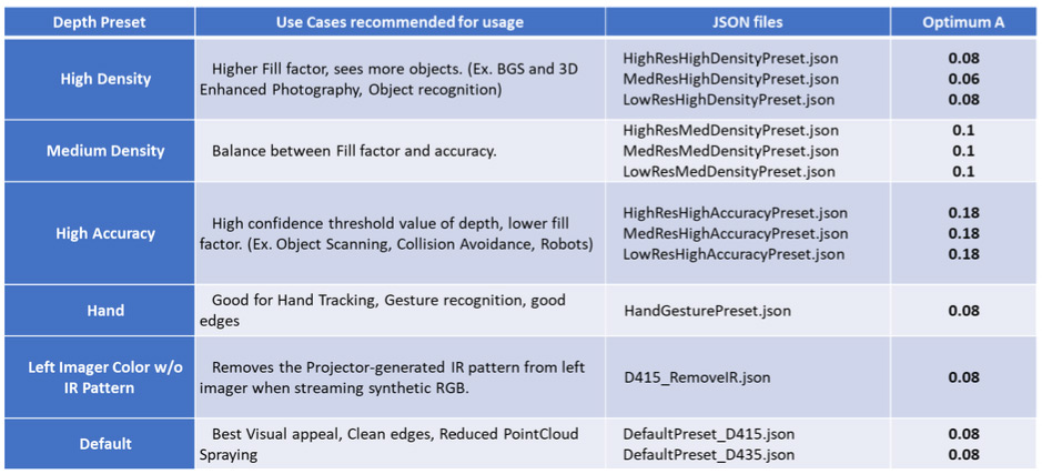
939 — Table 1. Table of optimum A-factors for each depth preset that improve the subpixel depth accuracy linearity. These are also found here: https://github.com/IntelRealSense/librealsense/wiki/D400-Series-Visual-Presets

There are a few interesting aspects to note. First, to observe and optimize for this effect, it is best to look at a small region of interest, and not the full field of view. This is because other effects such as the target linearity or lens calibration may affect the observed measurements. For ranges below 2m we also recommend setting the depth units to 100, instead of the default 1000. This allows for depth to be reported in units of 100 μm instead of 1 mm.

Second, if one measures the concurrent RMS Error of the depth, or the standard deviation of plane fit of a small ROI, as a function of range, then one may observe the behavior shown in bottom graph of Figure 2. This graph shows spikes in the RMS values at values that correspond to Half-Disparities, which is why we also sometimes refer to this the phenomenon as the half-disparity issue. As we use a more optimal A=0.08, we see that the overall average RMS value increases, but that the half-disparity spikes diminish or disappear. One may be tempted to think that since the RMS value is smaller overall for A=0 (ignoring the spikes), that this would be a preferred settings. This is incorrect. The smaller RMS values are a deleterious effect, also sometimes called pixel-locking. Consider the extreme case of no subpixel behavior. In this case all depth values would have to correspond to discrete disparities. When the actual distance to an object is between disparities, the disparity will lock to the nearest discrete value. This value will clearly be wrong, but the RMS error could still in this case be incorrectly reported as near 0. At the half disparity distance, depth values would suddenly become very noisy as they jump between adjacent disparities. This is what leads to the spikes. In short, measuring a fairly uniform distribution of RMS Error as a function of depth is a sign of a good depth setting and camera.

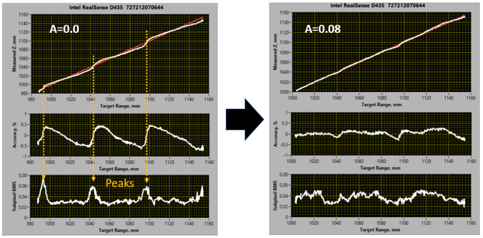
943 — Figure 2. Same measurement as Figure 1, but with the addition of the RMS Error measurement at the bottom. This graph shows spikes in RMS values that correspond to “Half disparities”. For A=0.08 the RMS error with distance becomes much more uniform, and does not artificially suppress the noise between half disparities.

We have focused these discussions on the D435. We have found that the D415 behaves almost identically, so the same optimal values of A can be used.

Finally, we consider what behavior one might expect across much larger depth ranges, if the A-factor is kept at 0. Figure 3 shows the expected theoretical behavior in the range from 200 mm to 4000 mm for the D435. As can be seen for the “High Density” simulation (left graph), the amplitude of the accuracy errors increases with distance away, exceeding +/-1.5% errors at 4 m. For “High Accuracy” the uncorrected depth oscillations reach +/-3.4%. This graph also serves to give an indication of the sampling interval one would need to have to fully characterize the effect. At 4 m range, a single disparity is 0.7 m, while at 20 cm range it is about 2 mm.

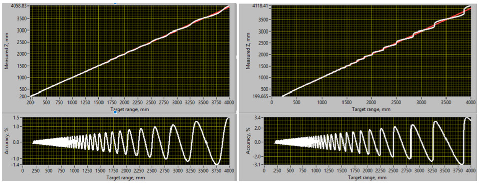
946 — Figure 3. The theoretical curves for the depth linearities for D435 for A=0, for High Density Present (Left) and High Accuracy Preset (Right). With correction of A=0.08, these oscillations are near zero.

Programming#

The A-factor can be set in a number of different ways:

Directly in the Intel RealSense Viewer.
By loading in a new JSON file with modified A-factor.
By using the open-source Intel RealSense SDK 2.0¹ to set the advanced parameters.

Figure 4 shows a screenshot of the Intel RealSense Viewer highlighting how to control the parameter.

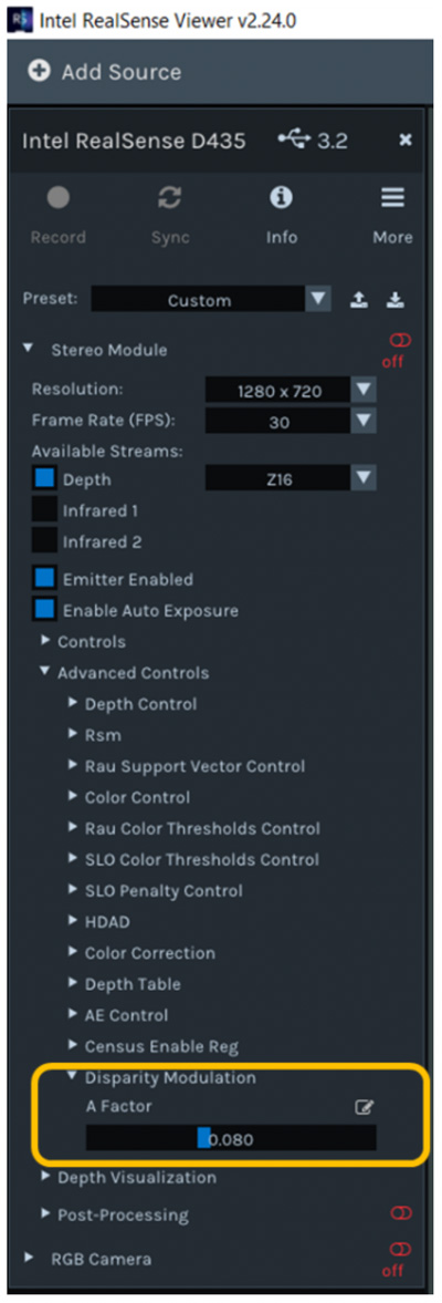
400 — Figure 4. Intel RealSense Viewer showing how to adjust the A-factor under the advanced settings.

The Intel RealSense API command is similar to other Advanced Settings commands. User can either use C or C++ APIs to set and get A-factor:

For C APIs, two new APIs are added:
RS2_Set_A-factor
RS2_Get_A-factor
For C++ APIs, a new struct DepthControlGroup is introduced, and two new member functions are added in the advanced_mode class:
set_new_depth_control
get_new_depth_control

Conclusion#

We have presented a series of measurements that show that the D435 and D415 cameras exhibit some non-linear depth accuracy behavior on a sub-pixel disparity scale. We have shown how the depth measurement linearity can be improved by 3-4x but using a new parameter called the A-factor, which has been introduced in new Firmware and the Intel RealSense SDK 2.0 as an advanced depth setting². The A-factor has now been incorporated into new JSON depth preset files, but the firmware has kept the default A=0.

References:

Intel RealSense SDK 2.0: https://github.com/IntelRealSense/librealsense
A-factor is supported in FW 5.11.06.250 and in RS SDK 2.24.0 or later.